


The generation of visually relevant, high-quality sounds is a longstanding challenge of deep learning. Solving this challenge would allow sound designers to spend less time searching large foley databases for the sound that is relevant to a specific video scene. Despite promising results shown in [1, 2, 3, 4], generation of long (10+ seconds) and high-quality audio samples supporting a large variety of visual scenes remains to be a challenge. The goal of this work is to bridge this gap.
To achieve this, we propose to tame the visually guided sound generation by shrinking a training dataset of audio spectrograms to a set of representative vectors aka. a codebook. Similar to word tokens in language modeling, these codebook vectors can be used by a transformer to sample a representation that can be easily decoded into a spectrogram. To employ visual information during sampling, we represent video frames as tokens and initialize the target sequence with them. This allows us to sample the next codebook token given the visual information and previously generated codebook tokens. Once autoregressive sampling is done, we remove the visual tokens from the sequence and reuse the pre-trained decoder part of the codebook autoencoder to decode the sampled sequence of codebook tokens into a sound spectrogram.
The natural format of audio is a waveform, a 1D signal resampled at tens of thousands of Hz. One option is to train a codebook directly on such waveforms and, then, sample the codes from it. Using this approach, OpenAI Jukebox could generate high-quality musical performances based on lyrics, style, and artist conditioning. Despite truly wonderful results, the sampling speed is rather slow (1 hour per 10 secs of generated audio).
Therefore, for efficiency, we operate on spectrograms, a condensed 2D representation of an audio signal which could be easily obtained from a raw waveform and inverted back to it. This also allows us to operate with sound as with images and draw on architectural elements from conditional image generation. In this work, we train a codebook on spectrograms similar to VQGAN (a variant of VQVAE) that proved to possess strong reconstruction power from smaller-scale codebook representations when applied to RGB images.
Once we can reliably reconstruct a spectrogram from a small-scale codebook representation we can train a model to sample from the pre-trained codebook a novel representation given visual conditioning. This representation can be then decoded into a new spectrogram relevant for visual input.
Next, we describe both the spectrogram codebook and the codebook sampler in detail.
The Spectrogram Codebook \(\mathcal{Z}\) is trained in an autoencoder with a quantized bottleneck:

The goal of the autoencoder is to reliably reconstruct the input spectrogram \(x\) from a small-scale codebook (quantized) representation \(z_\mathbf{q}.\) The codebook representation \(z_\mathbf{q}\) is obtained from the encoded representation \(\hat{z}\) just by looking up the closest elements from the codebook \(\mathcal{Z}.\) Both the Codebook Encoder (\(E\)) and Codebook Decoder (\(G\)) are generic 2D Conv stacks.
The training of the codebook is guided with four losses, two of which are traditional VQVAE losses: the codebook and reconstruction. The other two are inherited from the VQGAN architecture: patch-based adversarial and perceptual losses (LPIPS). The latter two losses were proven to allow reconstruction from smaller-scale codebook representations (see VQGAN).
Since the LPIPS loss relies on features of an ImageNet-pretrained classifier (VGG-16) it is not reasonable to expect that it would help to guide the generation of spectrograms. The closest relative of VGG-16 in audio classification is VGGish. However, we cannot make use of it because it: a) operates on 10 times shorter spectrograms than it is in our application, b) lack of depth and, thus, downsampling operations, in VGGish prevents extraction of large-scale features that could be useful in separating real and fake spectrograms. We, therefore, train from scratch a variant of VGGish architecture, referred to as VGGish-ish on VGGSound dataset. The new perceptual loss based on VGGish-ish is called LPAPS.
Transformers [1, 2, 3] have shown incredible success in sequence modeling. Once, the codebook representation is reformulated as a sequence, sampling from the codebook might benefit from the expressivity of a transformer. Such an approach has been shown to produce high-quality RGB images based on a depth, a semantic map, or a lower-resolution image in VQGAN. In this work, we propose to train such transformer to bridge two modalities, namely vision, and audio.
We train a variant of GPT-2 to predict the next codebook index given a visual condition in a form of visual tokens (features). The loss (cross-entropy) is calculated by comparing the sampled codebook indices \(\hat{s} = \{\hat{s_j}\}_{j=1}^{K}\) to the indices corresponding to the ground-truth spectrogram codebook representation \(z_\mathbf{q}\) (see the codebook figure ☝️).
On test-time, Transformer \(M\) autoregressively samples a sequence token-by-token primed with visual conditioning (frame-wise video features \(\hat{\mathcal{F}}\)) as follows:

When sampling of tokens is done, we cut out the visual tokens from the generated sequence and replace the predicted codebook indices \(\hat{s}\) with vectors from the codebook \(\mathcal{Z}\) to form the codebook representation \(\hat{z}_\mathbf{q}.\) We reshape the sequence \(\hat{s}\) into the 2D representation \(\hat{z}_\mathbf{q}\) in a column-major way. Then, we can decode this representation into a spectrogram by the pre-trained codebook decoder \(G.\) The generated spectrogram \(\hat{x}_\mathcal{F}\) can finally be transformed to a waveform \(\hat{w}\) with a pre-trained spectrogram vocoder \(V:\)

Overall, the Vision-based Conditional Cross-modal Sampler also includes the pretrained decoder from the codebook autoencoder \(G\) and a pretrained Spectrogram Vocoder \(V:\)

The most popular methods for vocoding a spectrogram are the Griffin-Lim algorithm and WaveNet. The Griffin-Lim algorithm is fast and can be applied to an open-domain dataset. However, the quality of the reconstructed waveform is dissatisfactory. At the same time, WaveNet allows to generate high-quality results but at the cost of sampling speed (20+ minutes for a 10-second sample on a GPU). Therefore, we train from scratch MelGAN on an open-domain dataset (VGGSound). This allows us to transform spectrograms to their waveforms in a fraction of a second on a CPU.
Human evaluation of content generation models is an expensive and tedious procedure. In the image generation field, this problem is bypassed with the automatic evaluation of fidelity using a family of metrics based on an ImageNet-pretrained Inception model. The most popular Inception-based metrics are Inception Score, Fréchet- and Kernel Inception Distance (FID & KID for short). However, automatic evaluation of a sound generation model remains an open question. In addition, our application requires the model to produce not only high-quality but also visually relevant samples. To this end, we propose a family of metrics for fidelity (quality) and relevance evaluation based on a novel architecture called Melception, a variant of Inception, trained as a classifier on a large-scale open-domain dataset (VGGSound).
For Fidelity evaluation of generated spectrograms, Melception can be directly adapted to calculate the whole range of Inception-based metrics including Inception Score as well as FID and KID. For automatic Visual Relevance evaluation, however, there are no well-defined metrics in the existing literature. To design one, we hypothesize that the class distribution of a generated spectrogram given a condition should be close to the class distribution of the original spectrogram for this condition. The class distributions for fake and real spectrograms can be formed by a pre-trained spectrogram classifier. To this end, we rely on Melception-based Kullback–Leibler divergence (MKL) as a measure of "distance" between two class distributions and average it among all samples in the dataset.
We demonstrate the generation capabilities of the proposed approach on two datasets with strong audio-visual correspondence: VAS and VGGSound. VAS is a relatively small-scale but manually curated dataset that consists of ~12.5k clips from YouTube. The clips span 8 classes: Dog, Fireworks, Drum, Baby, Gun, Sneeze, Cough, and Hammer.
VGGSound is a large-scale dataset with >190k video clips from YouTube spanning 300+ classes. The classes can be grouped as people, sports, nature, home, tools, vehicles, music, etc. VGGSound is 15 times larger than VAS but it is less curated due to the automatic collecting procedure. To the best of our knowledge, we are the first to apply VGGSound for sound generation.
Reliable reconstruction of input spectrograms is a necessary condition for high-quality spectrogram generation. We evaluate the reconstruction ability of the spectrogram autoencoder with the proposed set of metrics measuring fidelity (FID) and relevance (average MKL) of reconstructions. Moreover, such an experiment might give us a rough upper bound on the performance of the transformer. When compared to ground truth spectrograms, the reconstructions are expected to have high fidelity (low FID) and to be relevant (low mean MKL):
| Trained on | Evaluated on | FID ↓ |
Melception-based Kullback–Leibler divergence averaged among all samples in the dataset.
MKL ↓
|
|---|---|---|---|
| VGGSound | VGGSound | 1.0 | 0.8 |
| VGGSound | VAS | 3.2 | 0.7 |
| VAS | VAS | 6.0 | 1.0 |
The results imply high fidelity and relevance on both VGGSound (test) and VAS (validation) datasets. Notably, the performance of the VGGSound-pretrained codebook is better than of the VAS-pretrained codebook even when applied on the VAS validation set due to larger and more diverse data seen during training.
Next, we show qualitative results by drawing samples randomly from the hold-out sets of VGGSound and VAS and plot the reconstructions along with the ground-truth spectrograms.


_84b7NrzJWiI_420000_430000_x_id2379.jpeg)
_84b7NrzJWiI_420000_430000_xrec_id2379_vggsound_vqgan.jpeg)


We benchmark our visually guided generative model using three different settings:
a) the transformer is trained on VGGSound to sample from the
VGGSound-pretrained codebook,
b) the transformer is trained on VAS to sample from the
VGGSound codebook,
c) the transformer is trained on VAS to sample from the
VAS codebook.
We additionally compare different ImageNet-pretrained features:
BN-Inception (RGB + flow) and ResNet-50 (RGB).
As for spectrogram reconstruction evaluation, we rely on FID and average MKL as our metrics:
| Condition | FID ↓ |
Melception-based Kullback–Leibler divergence averaged among all samples in the dataset.
MKL ↓
|
FID ↓ |
Melception-based Kullback–Leibler divergence averaged among all samples in the dataset.
MKL ↓
|
FID ↓ |
Melception-based Kullback–Leibler divergence averaged among all samples in the dataset.
MKL ↓
|
The time (in seconds) it requires to sample a ~9.8-second audio.
Timer ↓
|
|
|---|---|---|---|---|---|---|---|---|
| No Features | 13.5 | 9.7 | 33.7 | 9.6 | 28.7 | 9.2 | 7.7 | |
| ResNet | 1 Feature | 11.5 | 7.3 | 26.5 | 6.7 | 25.1 | 6.3 | 7.7 |
| 5 Features | 11.3 | 7.0 | 22.3 | 6.5 | 20.9 | 6.1 | 7.9 | |
| 212 Features | 10.5 | 6.9 | 20.8 | 6.2 | 22.6 | 5.8 | 11.8 | |
| Inception | 1 Feature | 8.6 | 7.7 | 38.6 | 7.3 | 25.1 | 6.6 | 7.7 |
| 5 Features | 9.4 | 7.0 | 29.1 | 6.9 | 24.8 | 6.2 | 7.9 | |
| 212 Features | 9.6 | 6.8 | 20.5 | 6.0 | 25.4 | 5.9 | 11.8 | |
| Codebook | VGGSound |
VGGSound | VAS | |||||
| Sampling for | VGGSound | VAS | VAS | |||||
| Setting | (a) | (b) |
(c) | |||||
We observe that:
1) In general, the more features from a corresponding video are used,
the better the result in terms of relevance. However, there is a trade-off imposed by the sampling
speed which decreases with the size of the conditioning.
2) A large gap (log-scale) in mean MKL between visual and “empty” conditioning suggests the
importance of visual conditioning in producing relevant samples.
3) When the sampler and codebook are trained on the same dataset—settings (a) and
(c)—the fidelity remains on a similar level if visual conditioning
is used. This suggests that it is easier for the model to learn “features-codebook”
(visual-audio) correspondence even from just a few features. However, if trained on different
datasets (b), the sampler benefits from more visual information.
4) Both BN-Inception and ResNet-50 features achieve comparable performance, with BN-Inception
being slightly better on VGGSound and with longer conditioning in each setting.
Notably, the ResNet-50 features are RGB-only which significantly eases practical applications.
We attribute the small difference between the RGB + flow features and RGB-only features to the
fact that ResNet-50 is a
stronger
architecture than BN-Inception on the ImageNet benchmark.
Next, we show samples from all three different settings:

















Use our pre-trained model to generate samples for a custom video:
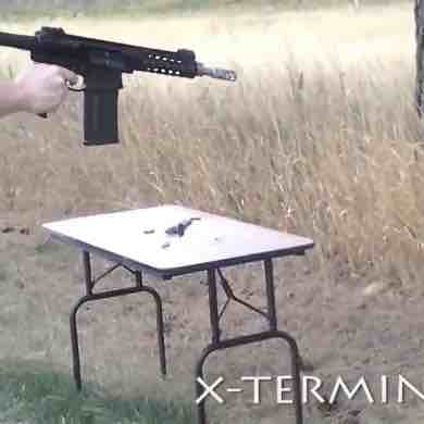







Note: the cough class in the VAS dataset has as few as 314 training videos videos







Note: the hammer class in the VAS dataset has as few as 318 training videos videos
We compare our model with RegNet, which is currently the strongest baseline in generating relevant sounds for a visual sequence. Since the RegNet approach requires training one model per class in a dataset, it explicitly shrinks the sampling space. On the contrary, our model learns to sample for all classes in a dataset at the same time which is a harder task. For a fair comparison, we will pass a class label (cls) along with the visual features into the model conditioning:
| Model | Parameters | FID ↓ |
Melception-based Kullback–Leibler divergence averaged among all samples in the dataset.
MKL ↓
|
The time (in seconds) it requires to sample a ~9.8-second audio.
Timer ↓
|
|---|---|---|---|---|
|
Ours
(b): The transformer is trained on the VAS dataset to sample from a
VGGSound-pretrained codebook
(b)
| 379M | 20.5 | 6.0 | 12 |
| Ours
(c): The transformer is trained on the VAS dataset to sample from a VAS-pretrained
codebook
(c)
| 377M | 25.4 | 5.9 | 12 |
| RegNet |
RegNet approach requires to train one model per class. There are 8 classes in VAS.
8\(\times\)
| 78.8 | 5.7 | 1500 |
| Ours
(b): The transformer is trained on the VAS dataset to sample from a
VGGSound-pretrained codebook
(b)
| 379M | 20.2 | 5.7 | 12 |
| Ours
(c): The transformer is trained on the VAS dataset to sample from a
VAS-pretrained codebook
(c)
| 377M | 24.9 | 5.5 | 12 |
According to the results, our model significantly outperforms the baseline in terms of fidelity (FID) while being on par or better in generating relevant samples. Moreover, the models without the cls token have competitive performance with RegNet. This suggests that our model is able to learn the mapping between the visual features and the class distribution through the "features-codebook" correspondence. We highlight that our model is trained on all dataset classes at once which is a much harder requirement than the baseline.










The following results show the capability of a model to generate samples without visual condition which, essentially, depicts how well the model captures the distribution of the training set. Both the codebook and the transformer are trained on the same dataset and the samples are not cherry-picked.


The transformer, given the previously generated part of the sequence, samples the next token. Here, we show the ability of the model to seamlessly continue a sequence of codebook indices from the original audio. The samples are drawn randomly from the hold-out sets and are not cherry-picked.


Note: the cough class in the VAS dataset has as few as 314 training videos videos


Temporal diversity is an important factor of high-fidelity audio. At the same time, it is challenging to generate a diverse but relevant sample which imposes a trade-off. The on-the-surface approach to sample the next item in the sequence is to always pick the codebook item that was predicted with the highest probability of being the next. This approach, however, will result in generating relevant but unpleasant, unnatural, and low-diversity samples.
To avoid it, we can use the distribution for the whole vocabulary (codebook) instead of the top one alone. These distributions can form weights for a multinomial distribution. This simply means that the larger the probability for the item, the more likely it will be picked as the next one.
However, we found that allowing the transformer to sample from all available codebook items indeed improves diversity but, at the same time, deteriorates relevance. Therefore, we end up in the "relevance-diversity" trade-off. To somewhat mitigate this issue, we control the trade-off by clipping the distribution. In particular, instead of either picking only the top one or use all available codebook items, we clip the set of available items to the Top-\(X\) according to their predicted probabilities.
Next, we show how this observation can be used to control the sample diversity:


or quantitatively relying on Melception-based FID and average MKL (the lower the better):
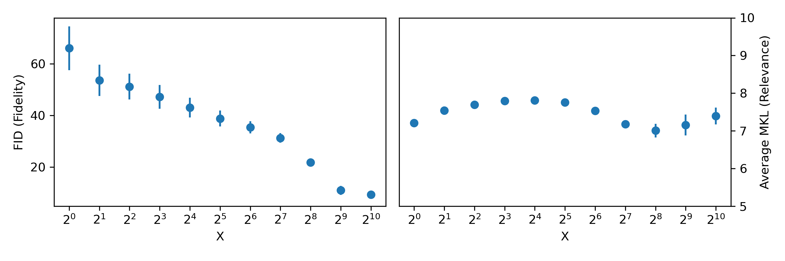
An ideal conditional generative model is expected to produce relevant examples for every class in a dataset. Here we show how relevant the generated samples are across every class in the VGGSound dataset:

Despite that model performance on a majority of the classes fall into [7 ± 0.7] interval of the MKL yet there is still room for improvement in the capabilities of a model to handle multiple classes which we hope to see in future research.
Since the generation of a relevant sound given a set of visual features is an ill-posted problem, a model is expected to produce a variety of relevant samples for the same condition. We show that our model is capable of generating a variety of relevant samples for the same visual condition:






Given the provided visual sequence ("a person is talking with a crowd on the background"), it is difficult to guess why the person turned back to the crowd, e.g. because they were "cheering" or "booing". At the same time, we also notice the limitation of the model, i. e. sometimes it confuses the gender or age of a person. However, we believe these are reasonable mistakes considering the difficulty of the scene.
A recent (July, 2021) ArXiv submission, show-cased a VQVAE with the adversarial loss, called SoundStream, on lossy compression of a waveform and reported the state-of-the-art results on the 3 kbps bitrate, which is designed for music and speech datasets. Since our approach includes sampling from a pre-trained codebook, we can employ our Spectrogram VQGAN pre-trained on an open-domain dataset as a neural audio codec without a change. Our approach allows encoding at, approximately, 0.27 kbps bitrate with the VGGSound codebook and 0.19 kbps with the VAS codebook.
We provide a small qualitative comparison of reconstructions of Lyra (only speech), SoundStream (only speech and music), and Spectrogram VQGAN (open-domain). We will use the same 3-second samples as provided on the SoundStream project page since the source code for the SoundStream has not been released to the public (checked on 20 October, 2021; the authors promised to release it as a part of Lyra toolbox).
As a result, despite having one order of magnitude smaller bitrate budget, Spectrogram VQGAN achieves comparable performance with SoundStream in reconstruction quality on music data and produces significantly better reconstructions than Lyra. However, as we observed before (Section 4.2 in the paper), Spectrogram VQGAN struggles with the fine details of human speech due to the audio preprocessing (mel-scale spectrogram) and absence of narrow domain pre-training as in Lyra and SoundStream. We highlight that Spectrogram VQGAN is trained on an open-domain hundred-class dataset (VGGSound) while SoundStream is trained on music and speech datasets separately.
Try our model on a custom audio on Google Colab:
Or with an even simplier interface without any exposed code:

Funding for this research project was provided by the Academy of Finland projects 327910 & 324346. We also acknowledge CSC – IT Center for Science, Finland, for computational resources.